XMRig monitoring, part 2: read the dashboards

XMRig monitoring series

1. Collect and store metrics
2. Read the dashboards
3. Logs, alerts and troubleshooting

Part 2 explains how we read XMRig and host metrics in Grafana. It covers the measurement windows, counter behaviour and collection age behind the panels, followed by an individual screenshot for each collected metric.

The queries use the collector and metric names from Part 1. The configuration bundle contains the matching example dashboard. Its setup requirements and validation limits are described in Part 1.

The dashboard images are real Grafana captures from November 4, 2026. They show one selected miner from 14:00 to 20:00 UTC, including a closer view from 15:45 to 16:15 UTC. Its visible name has been replaced with Miner A, and surrounding navigation has been cropped. The plotted values, axes, time range and units have not been rewritten. These views do not show our full inventory. The cream and orange artwork is illustration, not telemetry.

Build XMRig panels that preserve the meaning of the data

Use a Grafana instance variable populated from your expected-miner inventory or miner metrics. A typical query variable is:

label_values(xmrig_api_up, instance)

Use a selector such as instance=~"${instance:regex}" for multi-select panels. Keep an inventory-based table as well, because a variable built only from live telemetry can eventually stop offering a missing host. Do not let discovery of current series define what ought to exist.

Hashrate: show the window you are looking at

XMRig exposes short, medium and longer hashrate measurements. Our collector maps the miner's three summary values to 10s, 60s and 15m, matching its hashrate reporting implementation. These are measurements produced by the miner before Prometheus samples them.

For an individual miner, select its instance and the short window:

xmrig_hashrate_hps{instance="miner-a",window="10s"}

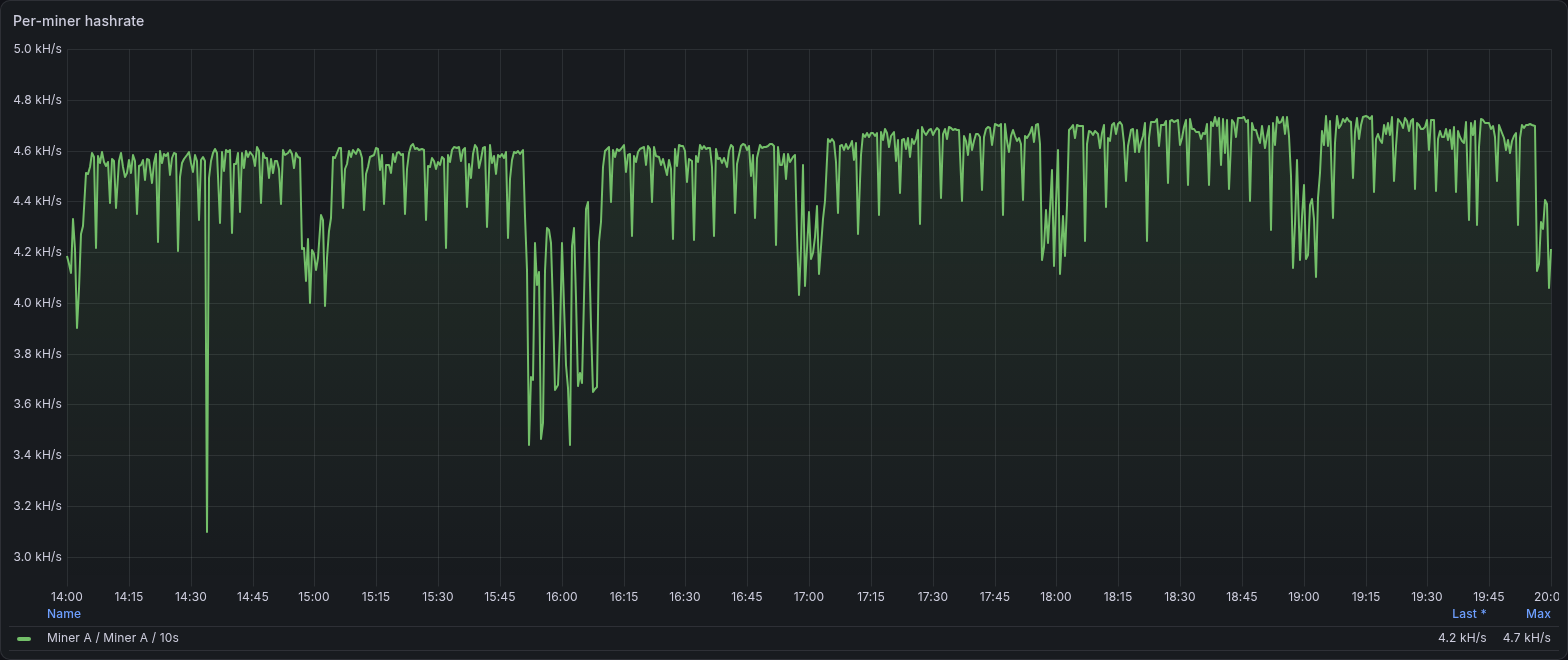
Miner A, November 4, 2026, 14:00 to 20:00 UTC. This is the individual hashrate panel filtered to one miner. The legend identifies the 10-second measurement window, and the vertical axis shows kH/s. Open the image to read it at full resolution.

The line spends much of this period near 4.6 to 4.7 kH/s, with brief drops and a longer disturbance around 16:00. A closer view makes that disturbance easier to inspect:

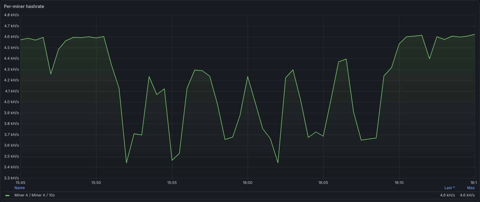
The same panel and miner, 15:45 to 16:15 UTC. Only the displayed time range has changed. The recorded series drops repeatedly to roughly 3.4 to 3.7 kH/s before returning near 4.6 kH/s around 16:10. This does not establish the cause.

Both screenshots use Grafana's automatic vertical scale. Neither axis starts at zero, and their lower bounds differ. Read the axis values when comparing the depth of a drop. The line connects sampled observations, so its shape does not expose every change between collections.

Compare that short window with the longer measurements:

xmrig_hashrate_hps{window="60s"}

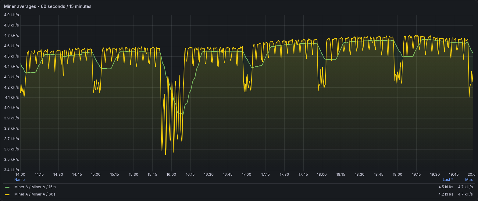
One miner, November 4, 2026, 14:00 to 20:00 UTC. The yellow 60-second line responds sharply to short changes. The green 15-minute line smooths and trails them. Both come from the miner's API.

The screenshot contains a pronounced dip around 16:00 UTC. The longer window stays depressed after the shorter one recovers because it still includes earlier measurements. That delay is expected from the window and should not be mistaken for a second incident.

A 30-second scrape of a 10-second rolling estimate is not a continuous record of every hash produced between scrapes. Increasing Grafana's refresh frequency cannot recover observations that were never collected. Choose a scrape interval and query resolution that fit the question, and preserve the window in the legend.

For a fleet total, sum a single window across distinct miners. Exclude proxy estimates and duplicate ingestion jobs. A miner's self-reported hashrate and a proxy's share-derived estimate can describe the same work from different vantage points. Adding them together would count that work twice.

Accepted work: use a counter rate and the right unit

60 * rate(xmrig_accepted_shares_total[5m])

This returns accepted shares per minute over a five-minute rate window. Configure the panel unit as shares/min, not operations per second. During this review, we found that mismatch in the existing dashboard's accepted-share panel. The example query and unit here make the intended scale explicit.

Use a counter-aware rate calculation rather than subtracting adjacent samples by hand. Apply the rate to each miner before aggregating across miners so resets remain visible to the calculation. Prometheus documents reset handling and rate semantics in its query-functions reference.

Accepted-share counts also depend on share difficulty. A miner can submit fewer, harder shares without losing the same proportion of useful work. Compare a rate change with difficulty, hashrate and rejection data before calling it a performance loss.

Rejections: include enough observations

The example collector exports accepted and submitted counters. This expression estimates the recent rejected percentage:

100 * clamp_min(
  rate(xmrig_submitted_shares_total[15m])
  - rate(xmrig_accepted_shares_total[15m]),
  0
)
/ clamp_min(rate(xmrig_submitted_shares_total[15m]), 0.000001)

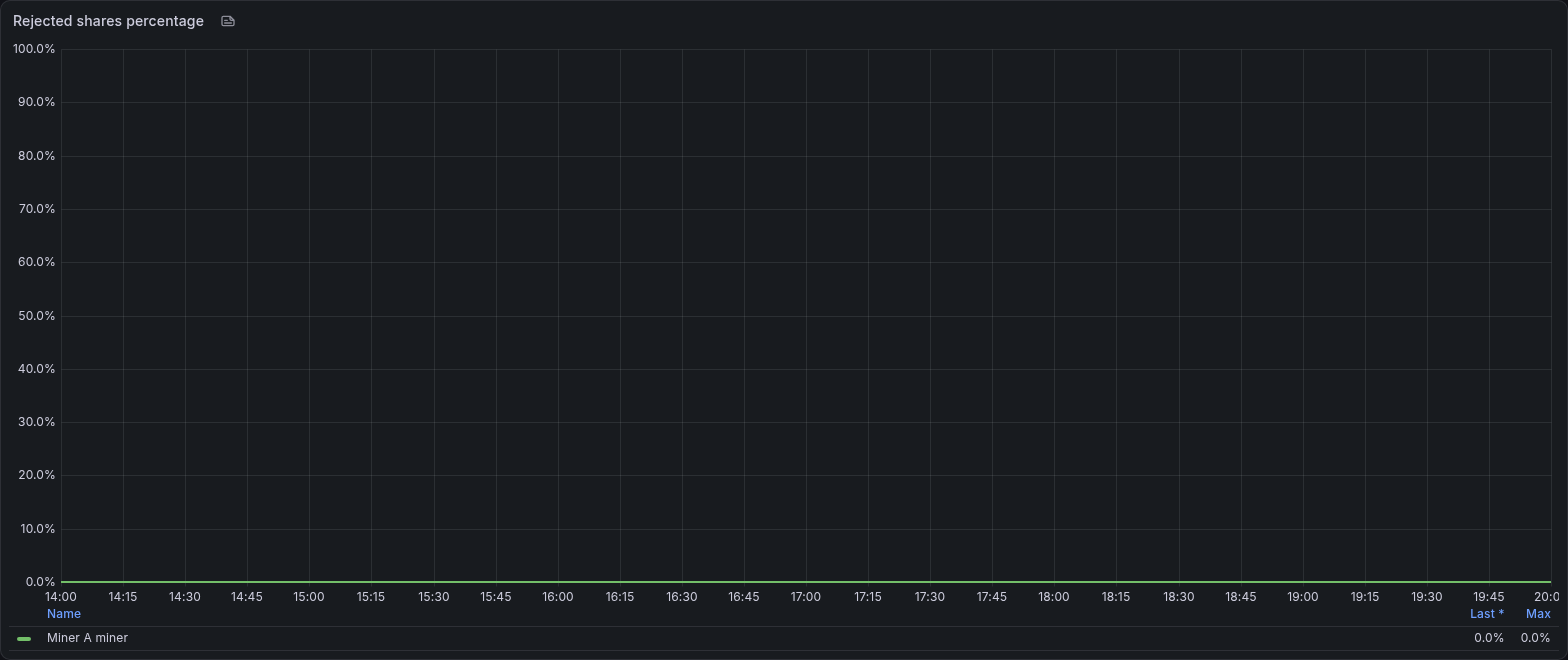
The existing dashboard's equivalent calculation shows zero rejected percentage for the selected miner in this interval. This is a six-hour observation of one miner, not a fleet-wide reliability claim.

The small denominator floor avoids division by zero, but it can also make a window with no submitted work display as zero percent. Pair the percentage with submitted-share volume. Zero rejects out of zero submissions is not a successful mining result.

A rejection alert should require both a sustained percentage and enough submissions to make it actionable. One rejected share out of one submission is 100 percent, but it is a weak basis for diagnosing a persistent connection problem. The example rules require more than ten submitted results in the window. That threshold is a starting point to tune, not a universal mining standard.

CPU and network: compare the host with the miner

A second dashboard places host CPU and network use side by side for the same miner and time range. Its network panel sums selected physical interface counters, including traffic from other applications.

For Linux Node Exporter data, this query gives average non-idle CPU time across the host's logical CPUs:

100 * (
  1 - avg by(instance) (
    rate(node_cpu_seconds_total{job="mining-hosts",mode="idle"}[5m])
  )
)

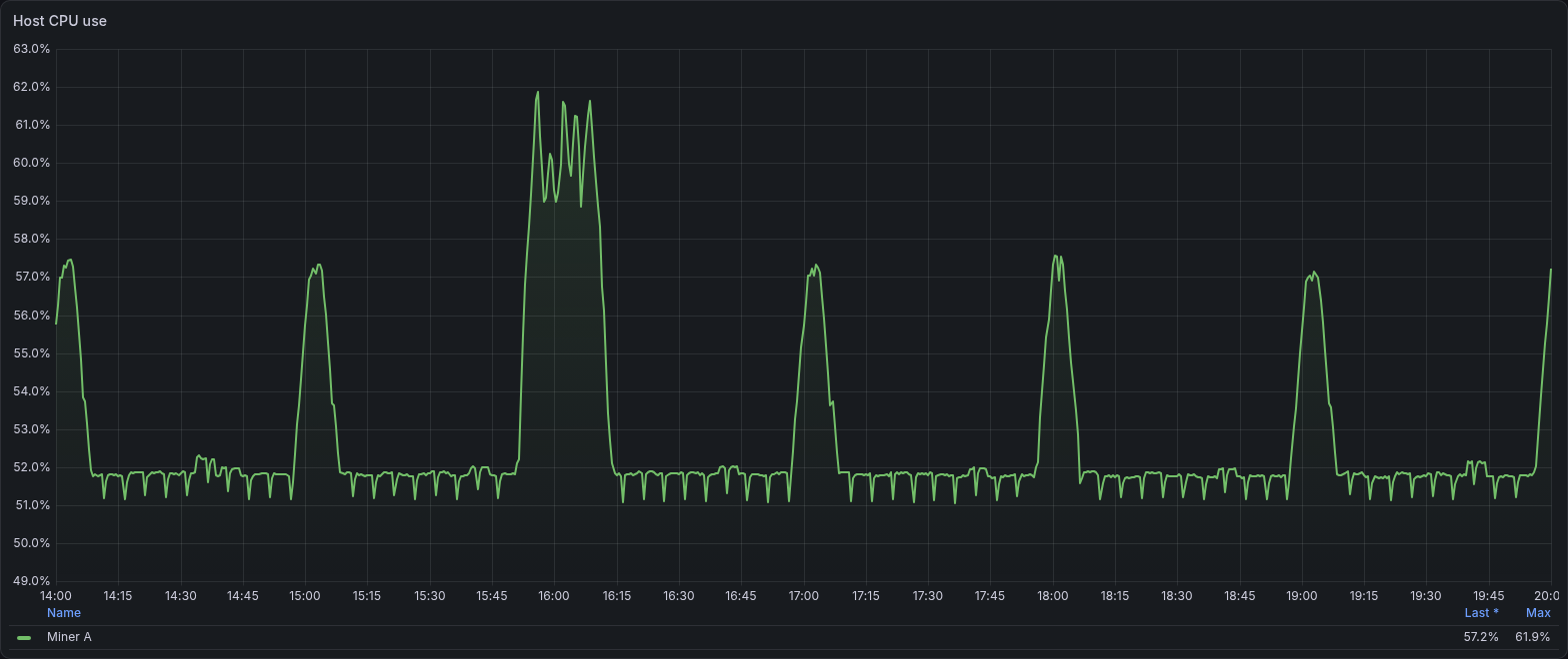
The five-minute CPU view rises during the same period as the hashrate dip. Competing host activity is one explanation to investigate with process-level evidence.

Do not infer that XMRig should use every logical CPU or that a lower host percentage is automatically waste. Thread placement, the workload and the machine's configuration affect the useful operating point. Use this panel to detect changes against that miner's normal behaviour.

For network throughput, choose the interface carrying the traffic you intend to measure, calculate a byte-counter rate, and multiply by eight for bits per second. Avoid summing a bridge, its member interface and a virtual interface carrying the same packets. Our host dashboard's selection is useful for host activity, but a traffic spike there could be a package download, backup or another application.

Temperature panels need similar care. Not every host exposes the same sensors. Label the chip and sensor, verify which measurement is meaningful, and leave unsupported sensors absent. A temperature increase is evidence to correlate with clocks, logs and hashrate, not a complete thermal-throttling diagnosis.

Latency: know what zero means

xmrig_pool_latency_milliseconds

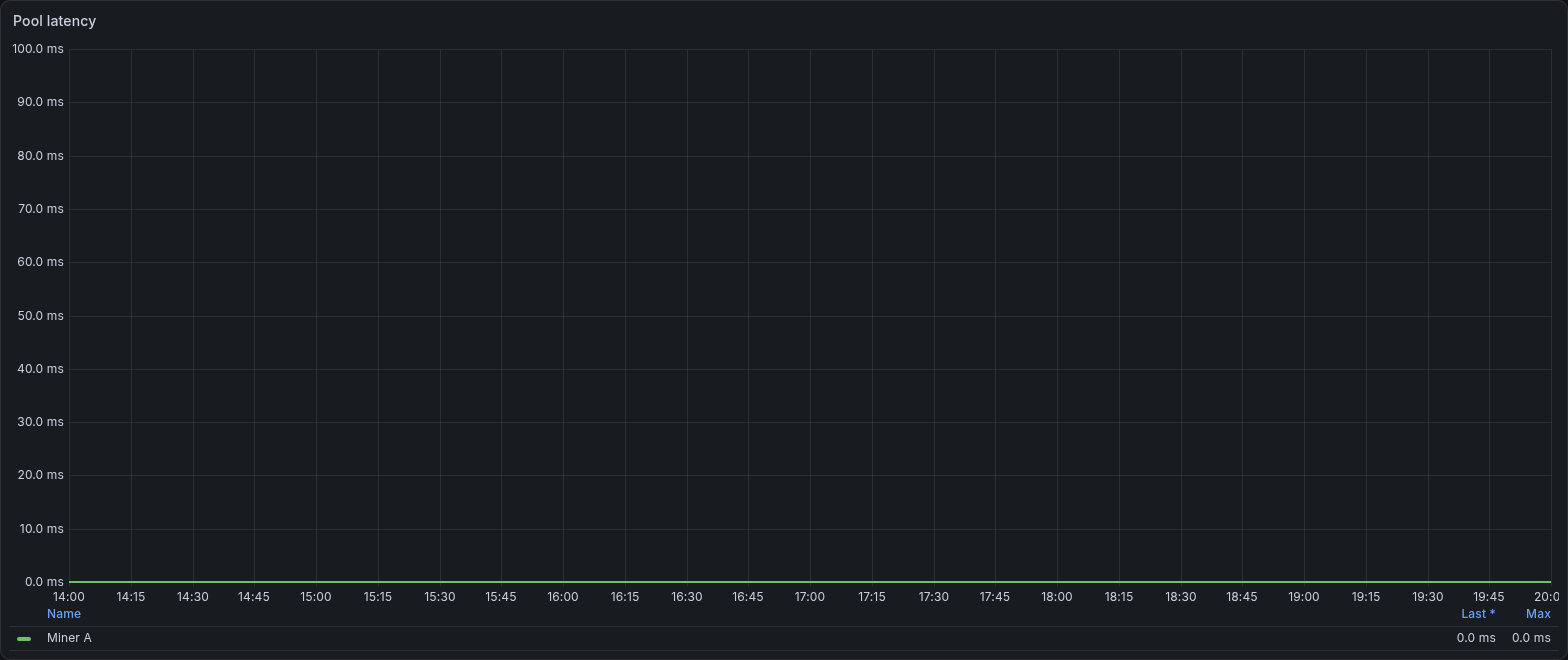
The inspected panel reports zero milliseconds from connection.ping for this interval. It is not an independently measured end-to-end network round-trip time. The production panel falls back to this field when results.latency is absent.

The example collector in Part 1 exports xmrig_pool_latency_milliseconds only when results.latency exists. That optional field is absent on the inspected miner, so this screenshot comes from the production exporter’s connection-ping series. Adapt the example mapping explicitly if you need the same view.

The screenshot is a useful limit on interpretation. A zero field is not proof of a physically instantaneous connection. Inspect the API field's meaning, measurement resolution and pool arrangement before treating it as network latency. If you need an independent latency or availability probe, collect one separately and give it a different name.

Freshness: graph the age of the measurement

time() - mining_collector_timestamp_seconds

Display this in seconds. It should remain near the expected collection and transport delay. A rising value says the collector's content is aging even if Node Exporter is still responding. Synchronize host clocks and alert on serious clock skew, because this expression compares timestamps from different machines.

Do not fill missing series with zero in Grafana. A missing hashrate could mean a new process has not completed its reporting window, an exporter stopped, an agent lost connectivity, or the host disappeared. The state needs its own label or panel. Connecting lines across a long gap can hide the period you most need to investigate.

A screenshot for each collected miner metric

The gallery covers all 20 XMRig metric families recorded for the selected miner in the inspected interval. It also covers the 20 host and collection-health families emitted by our custom exporters, plus the host CPU, memory, temperature, network, disk and filesystem views used here. The metric screenshot index maps each field to its screenshots and is also included in the configuration bundle.

The gallery covers metric families, using selected threads and devices for those measurements. It does not catalogue every Linux, container or monitoring-agent metric. Device names, version labels and the full thread inventory are omitted from the public views.

All panels use real recorded data from November 4, 2026, 14:00 to 20:00 UTC. Where a suitable panel did not already exist, we rendered a temporary, read-only Grafana view with descriptive titles and generic legends. These views were not saved over the operational dashboards. The source samples are unchanged, and every image opens at full resolution.

Optional fields need an explicit boundary. This miner did not emit separate results.accepted, results.rejected, results.invalid, results.expired, results.hashes_donate or results.latency series in this interval. The miner’s accepted and rejected work is represented by its share and connection counters. Proxy-specific worker and upstream metrics do not apply to this selected miner. Missing fields have not been turned into zero-valued graphs.

Miner state and uptime

Expected-source, API-health, metadata-presence and backend-enable gauges establish what is being monitored. Process and connection uptimes then help distinguish a miner restart from a reconnect.

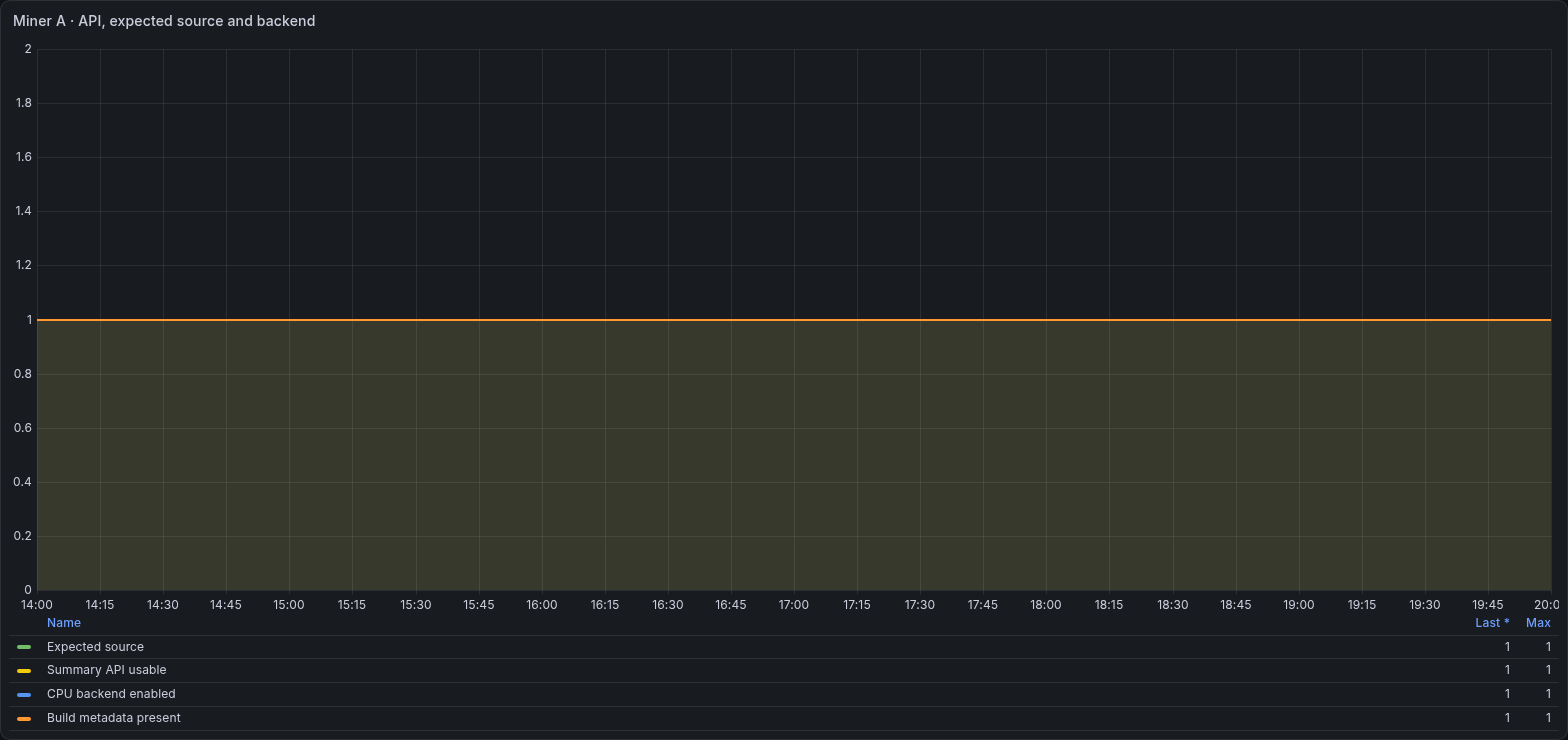
These are state gauges. A value of 1 reports the indicated state, not a hashrate. The metadata series carries version and algorithm labels in the private dashboard. Those labels are omitted here.

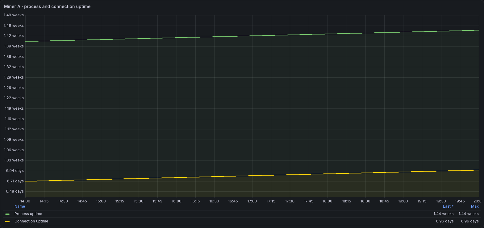
Process uptime and pool-connection uptime answer different questions. A reconnect can reset connection uptime while the mining process continues running.

Share accounting and pool work

These panels show the raw result and connection counters alongside their timing and difficulty fields. The definitions follow XMRig’s network-state implementation. The earlier latency screenshot covers connection.ping.

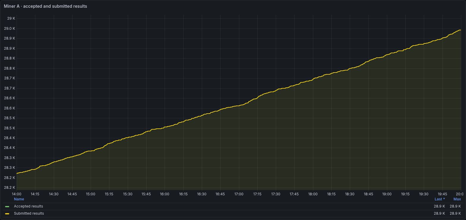
These are cumulative process counters, not shares per second. The submitted counter includes accepted and rejected results. Overlapping lines mean the two totals agree at the plotted samples.

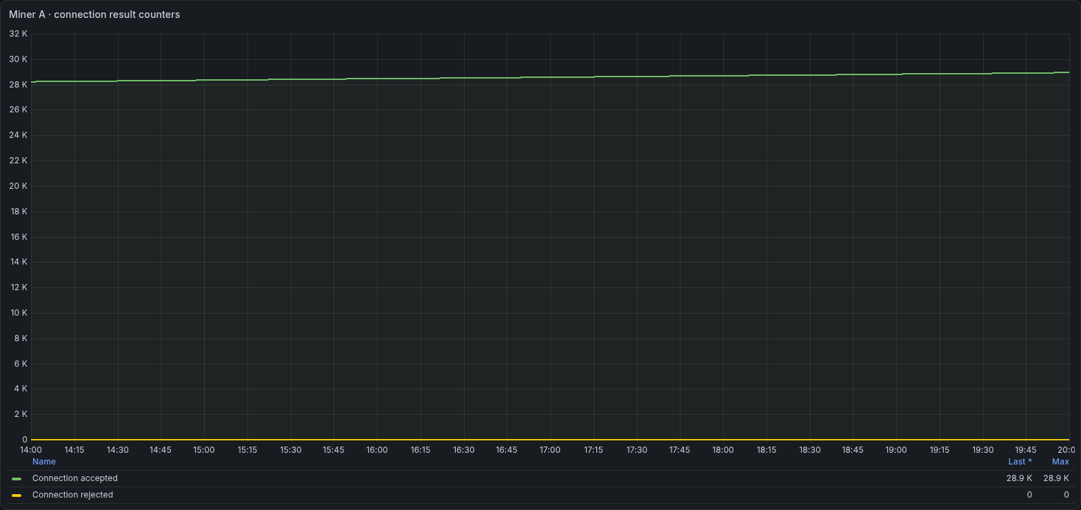
The connection object also exposes accepted and rejected counters. They are another view of the same result accounting, not extra work to add to the result counters.

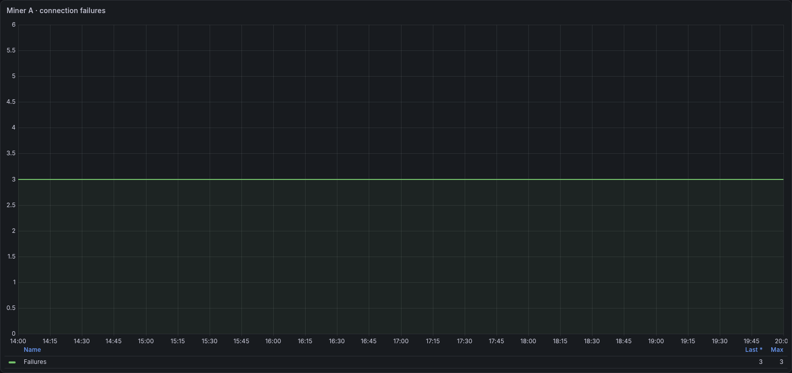
A failure counter complements connection uptime. Read increases and resets in context rather than interpreting an old cumulative total as a current outage.

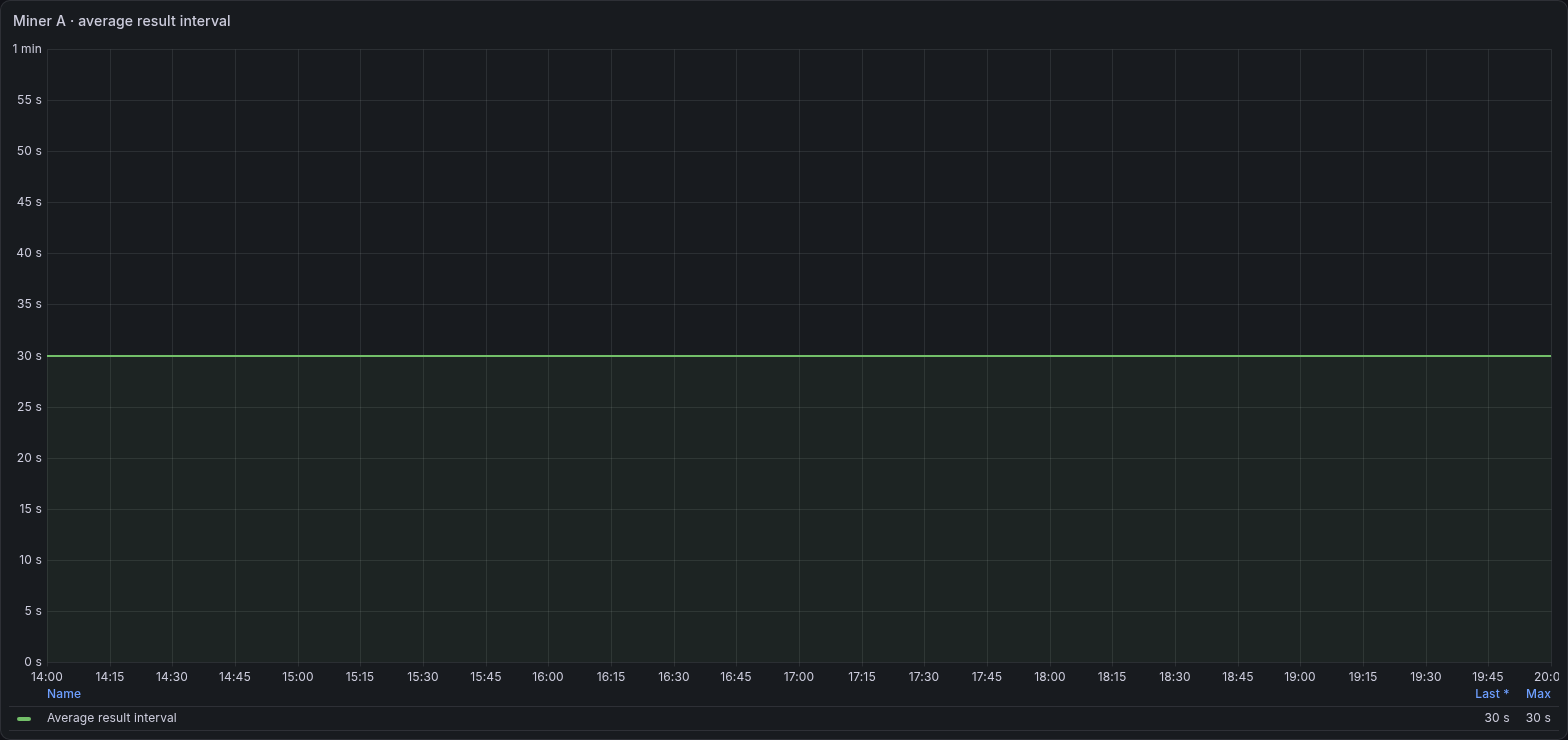
The API reports average result time in seconds. This is distinct from the millisecond response-time field shown in the pool-latency panel.

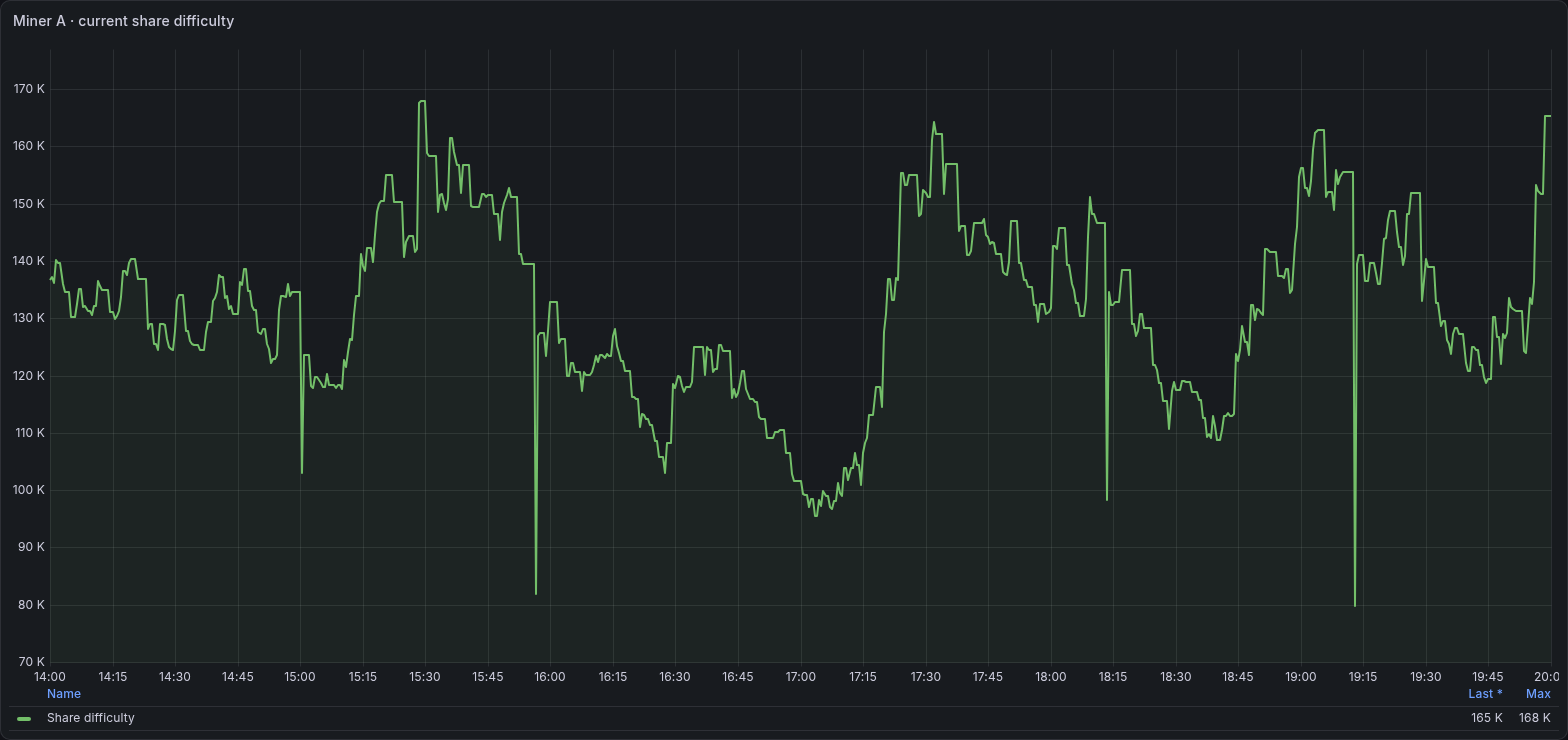
This is the difficulty of work assigned to the miner. It is not Monero main-chain network difficulty.

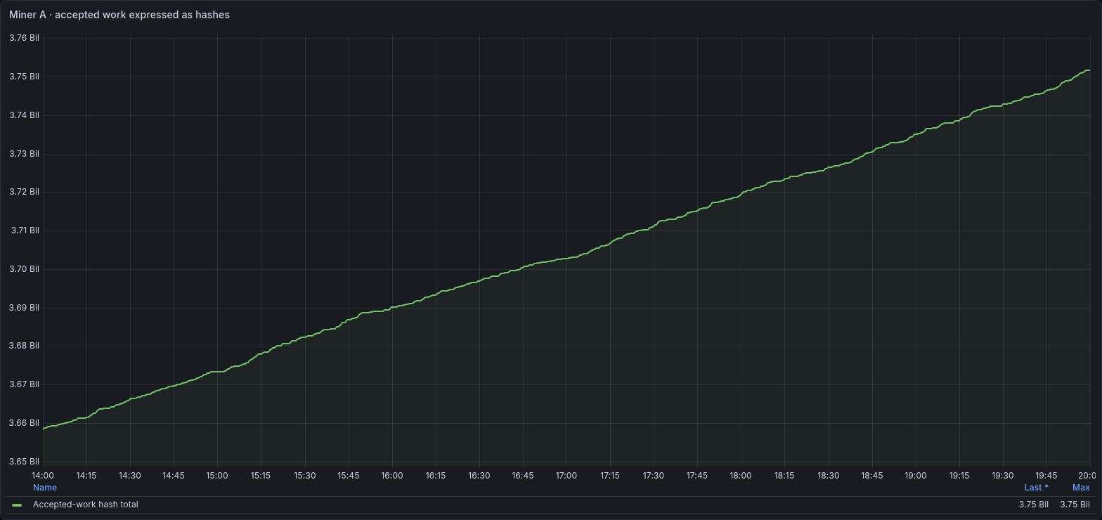
XMRig increments this total by the difficulty of accepted results. It is an accepted-work accounting measure, not a direct count of every CPU hash calculation.

Threads, huge pages and process memory

The total hashrate screenshots above cover all three miner windows. The following views add a selected thread’s three windows, huge-page counts and the process resident set.

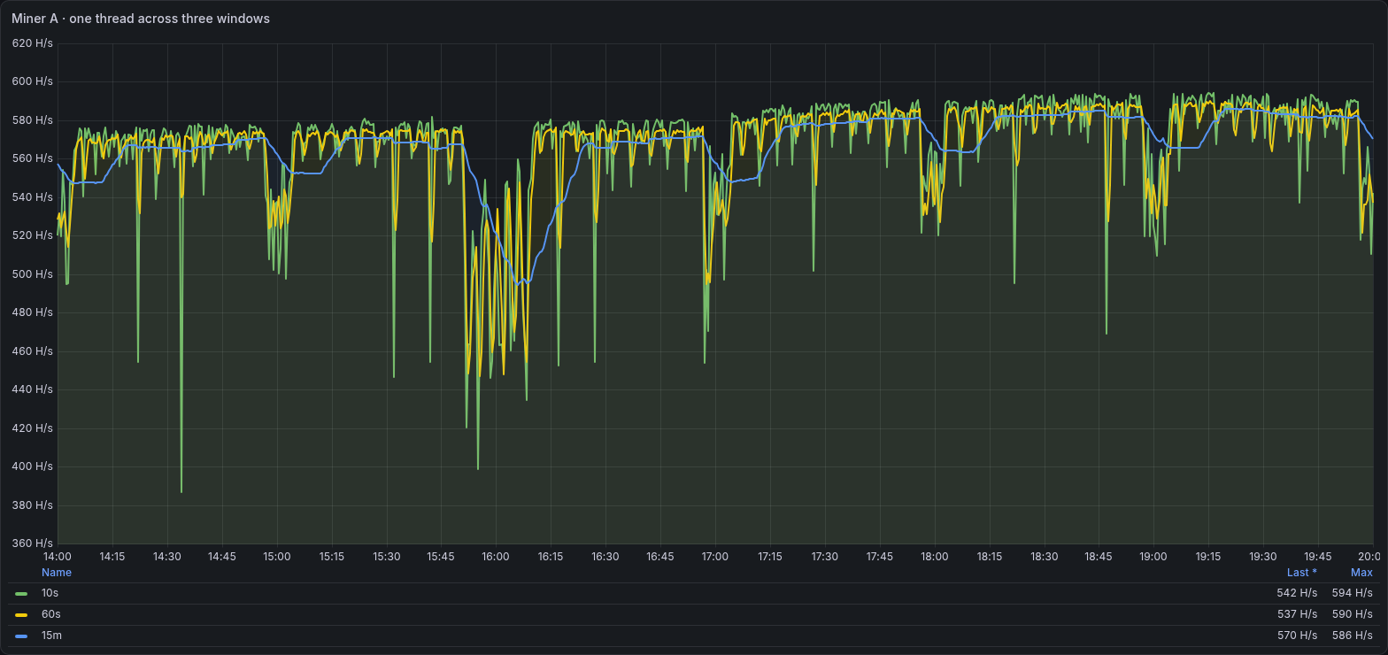
One selected thread, shown across the same three windows as the miner total. The thread identity is omitted. This illustrates the metric family without publishing the complete thread inventory.

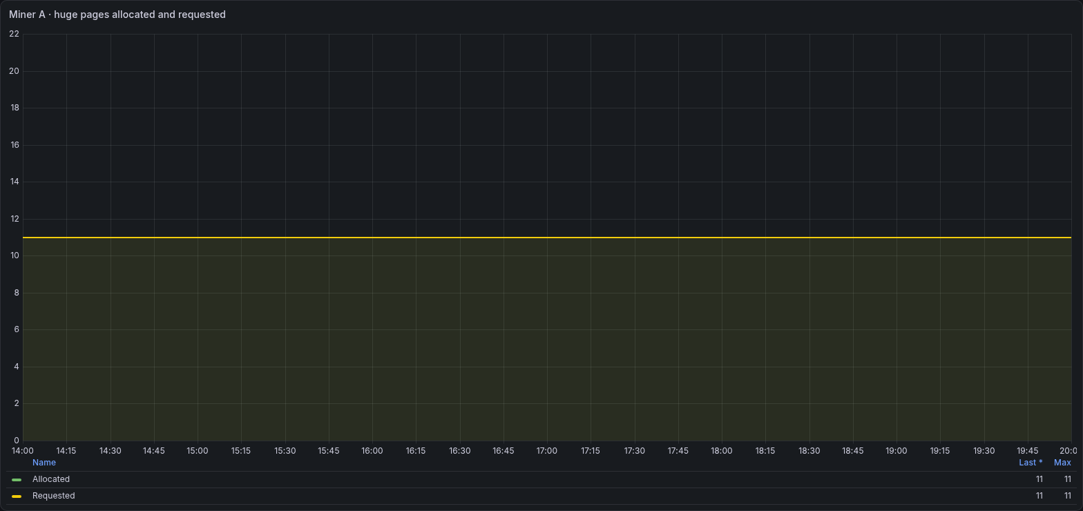
These are page counts. Compare allocated with requested before using an allocation percentage. Counts do not state a page size or a byte total.

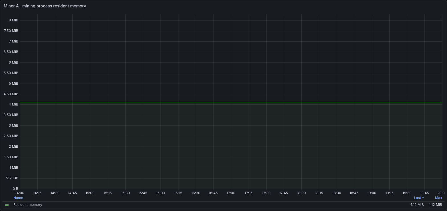
Resident memory belongs to the mining process. It is separate from total host memory use, filesystem cache and memory used by other processes.

Collector and transport health

These fields come from the monitoring collector. They explain whether the surrounding telemetry is recent and whether its authenticated transport needs attention.

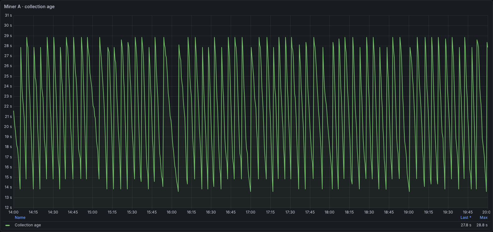
Age is computed from the collected timestamp. It makes stale output readable as elapsed seconds rather than as an epoch timestamp.

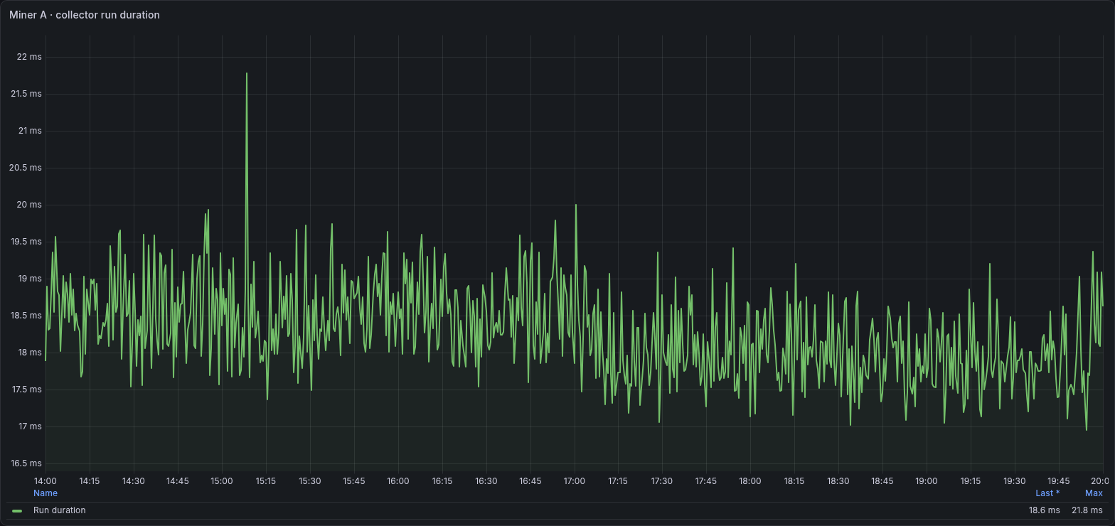
This is the full production collector run, which covers more than the smaller XMRig-only example. Its absolute duration should not be treated as a benchmark for that example.

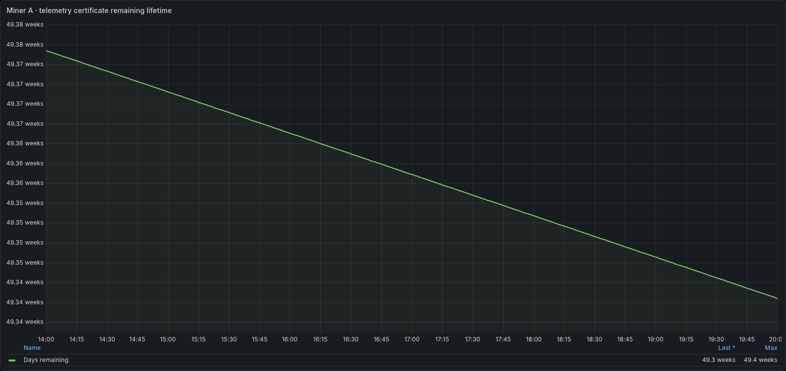
The collector exports certificate expiry as an epoch timestamp. This panel computes the remaining lifetime in days, which Grafana displays as weeks at this scale. It does not expose the certificate, subject or private key.

Host temperatures and CPU energy

These measurements describe the host around the miner. Keep sensor temperatures, energy and derived power in their respective units.

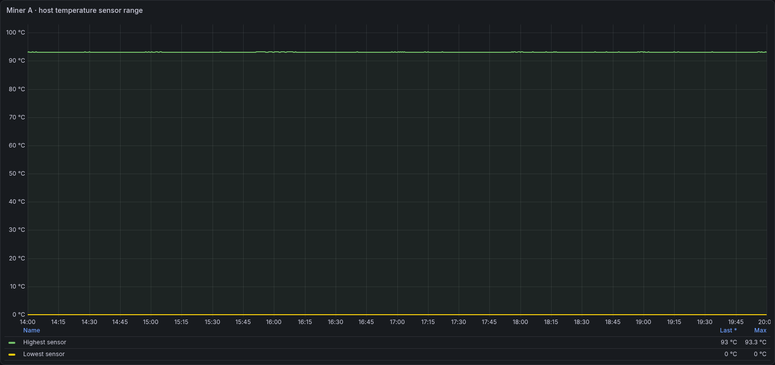
The bounds summarize the available host temperature sensors. They are not both CPU temperatures. A zero reading needs sensor validation before it can be treated as a physical temperature. Hardware sensor identities and the full device inventory are omitted.

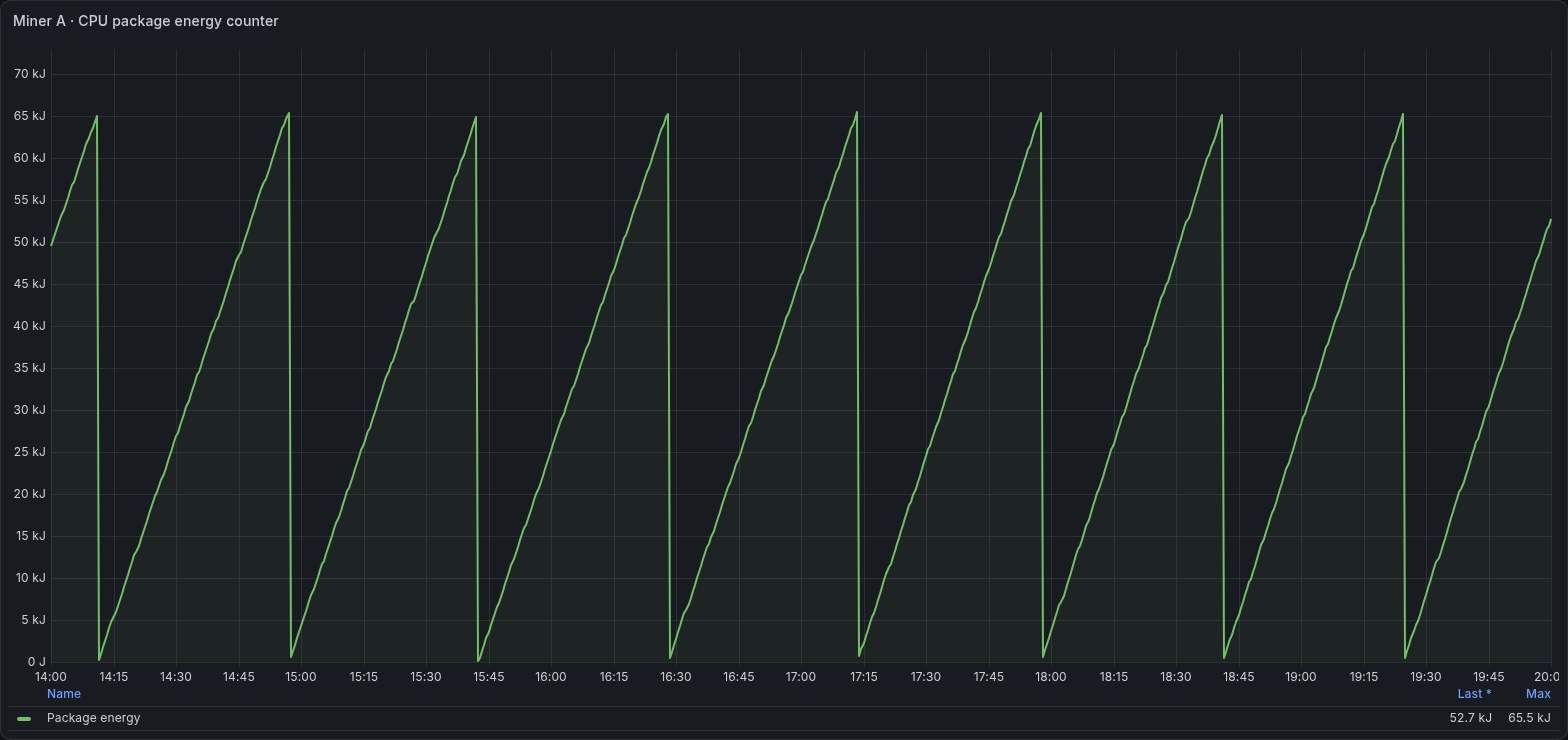
The collected value is cumulative energy in joules for the selected package domain. Counter rollover and resets need to be considered when deriving power.

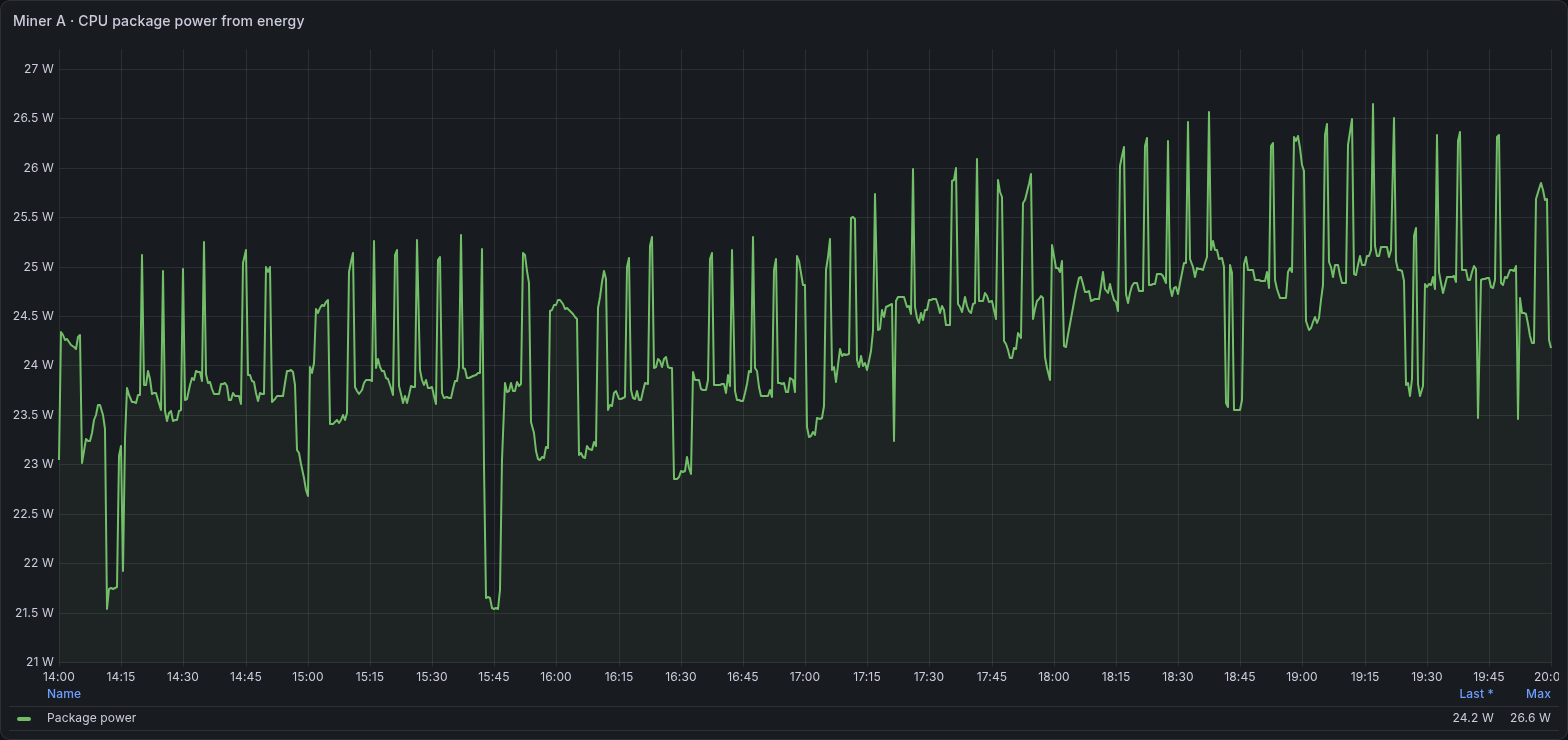
The five-minute rate of the energy counter estimates package watts. It excludes power outside the measured domain and is not a wall-meter measurement.

Host memory, network and storage activity

The earlier CPU screenshot covers processor utilization. These views add available memory, one physical network interface, one physical disk and one filesystem.

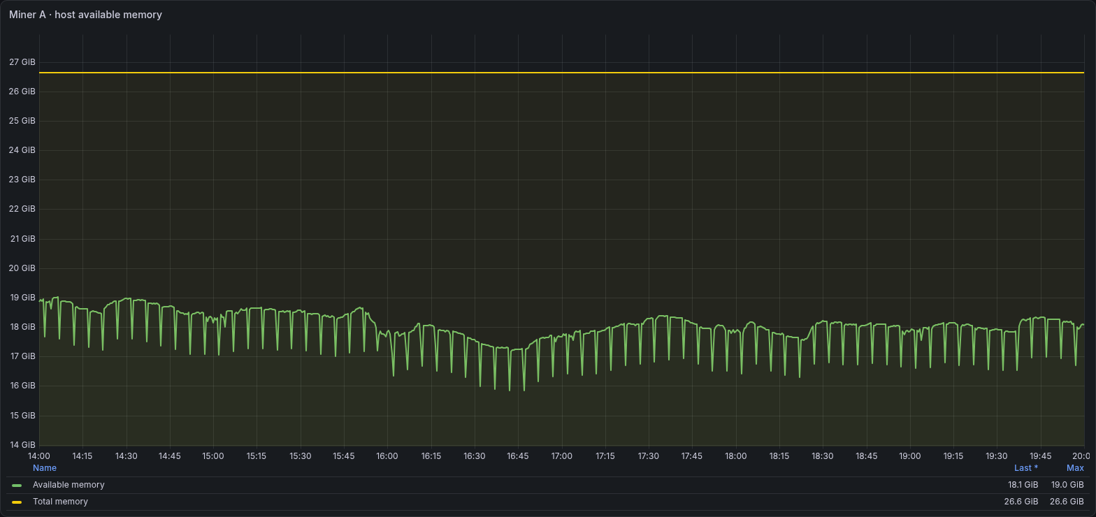
Available host memory is shown separately from the miner process resident set. The plotted values are real and are not rescaled to imply a different machine.

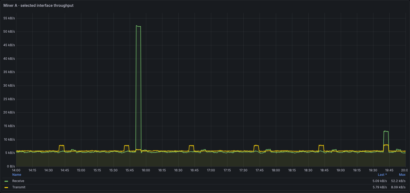
Receive and transmit rates use one selected physical interface. Summing bridges and virtual interfaces could count the same traffic more than once. The interface name is omitted.

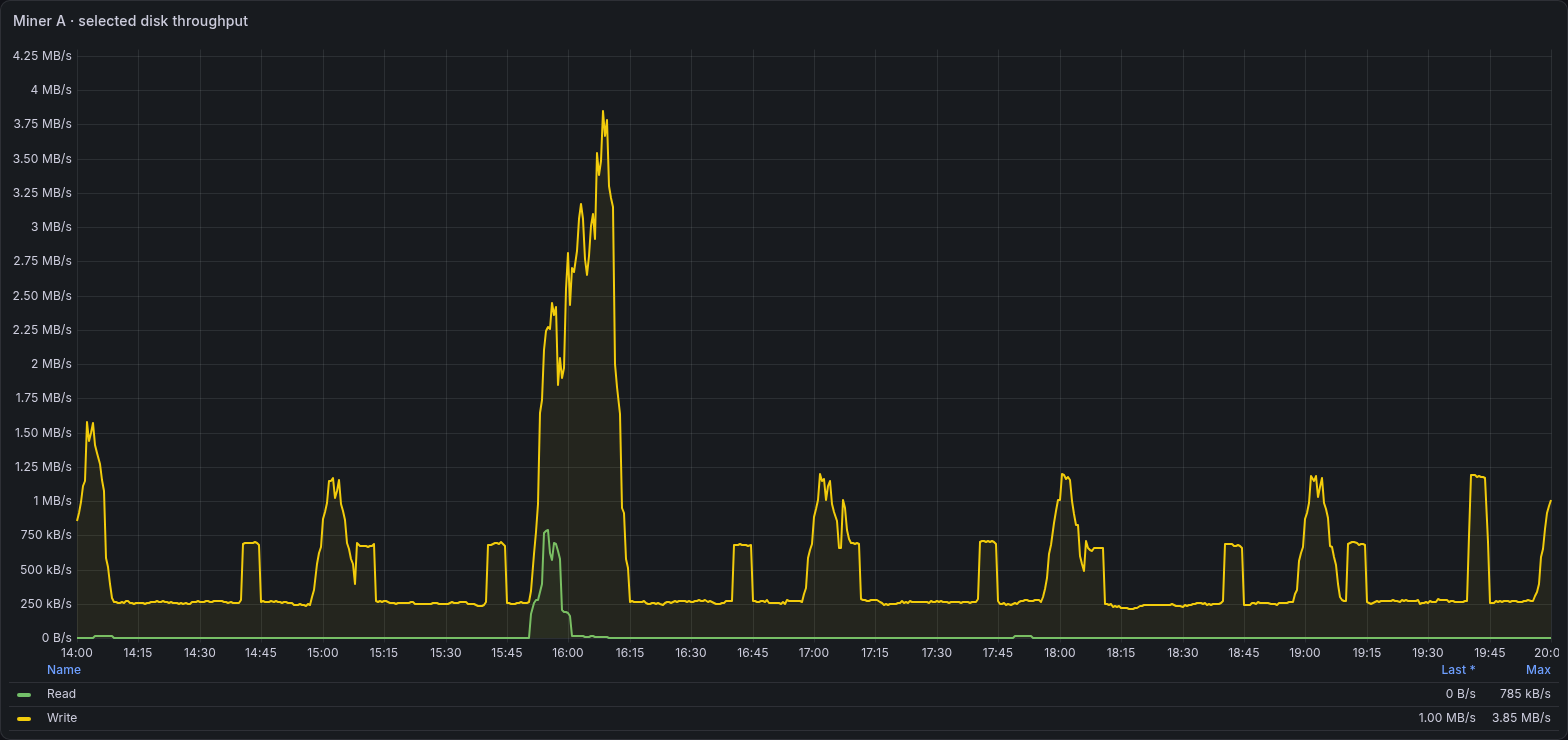
These are byte-counter rates for one selected physical disk. The device name is omitted, and the graph does not combine the physical disk with its mapped logical volume.

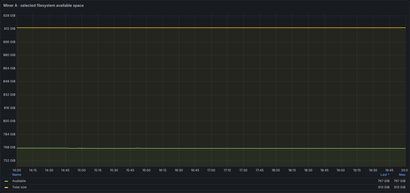
Available space and filesystem size describe the selected filesystem. Its device path and mount label are omitted.

Drive health and collection age

Drive health is collected separately from the XMRig API. Keep each drive-reported field in its own unit and check the drive-health timestamp before relying on it.

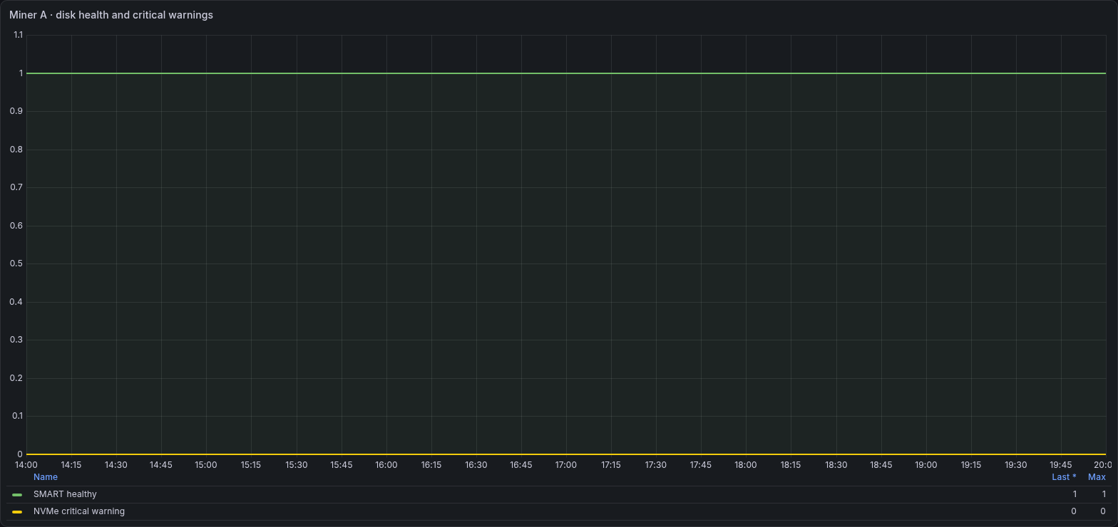
Health and critical-warning fields are shown as raw values. Their encodings differ. A healthy flag of 1 and a critical-warning value of 0 are not interchangeable scales.

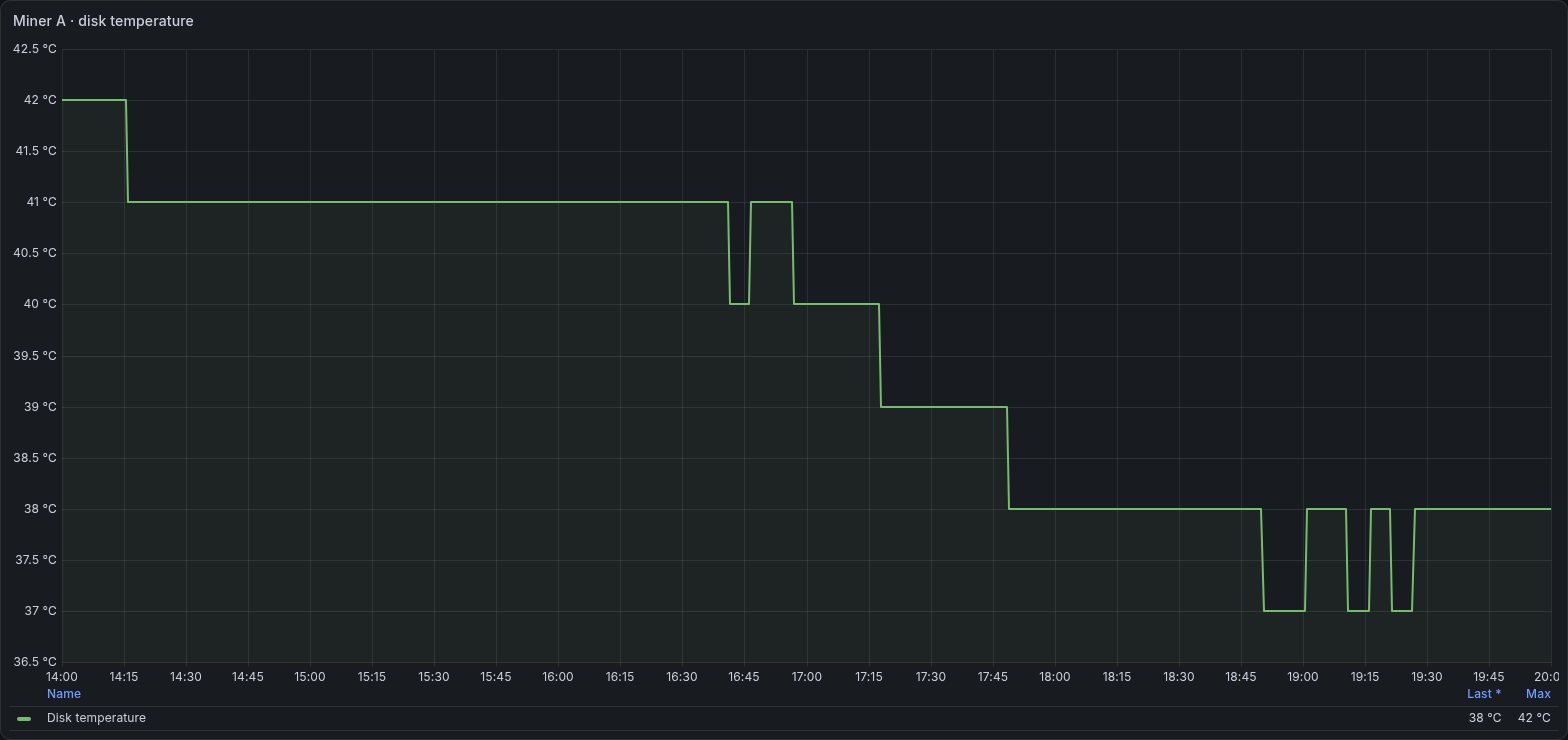
This is the selected disk temperature from the drive-health collector. It is separate from the summarized host sensor range.

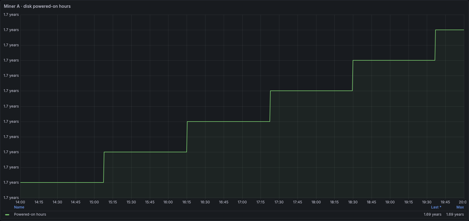
The drive-reported powered-on-hours counter describes device history. Grafana displays this duration in years at this scale. It does not measure the age or uptime of the current XMRig process.

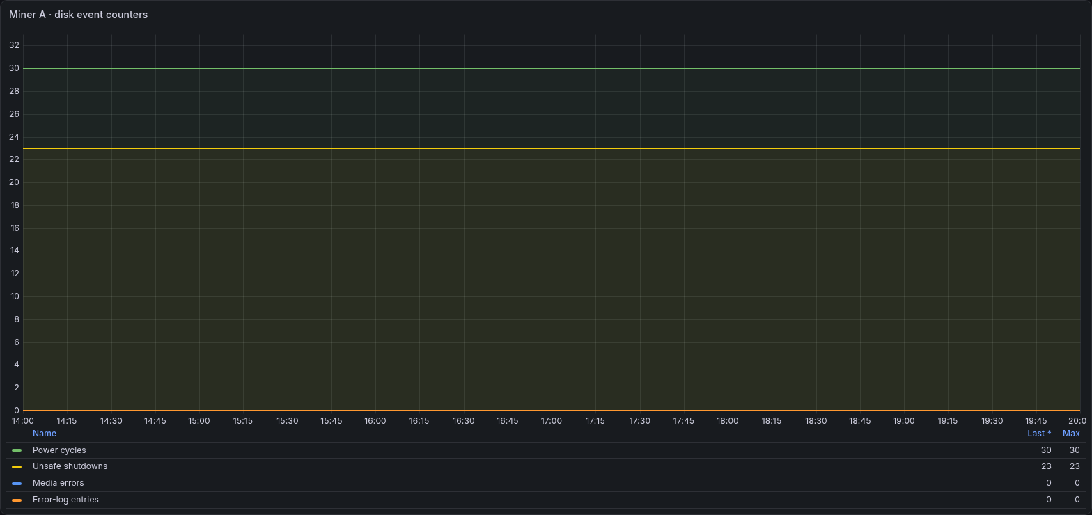
These are different cumulative drive event counters. Their totals are not an incident count for the selected six-hour window. Compare changes and consult the drive log when diagnosing them.

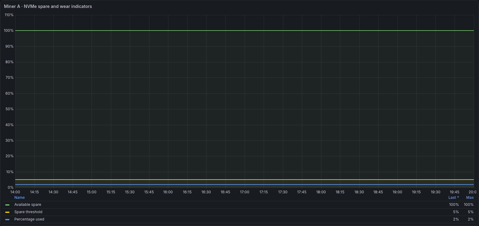
Available spare, its warning threshold and percentage used describe different drive-health properties. Percentage used is not filesystem occupancy.

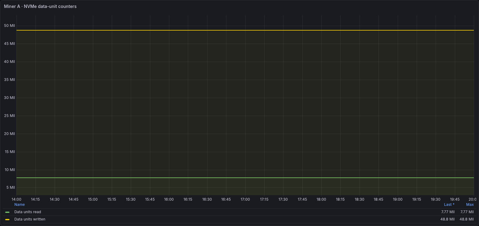
The raw drive data-unit counters are kept in their exported units. They are not labelled as bytes or converted using an assumed multiplier.

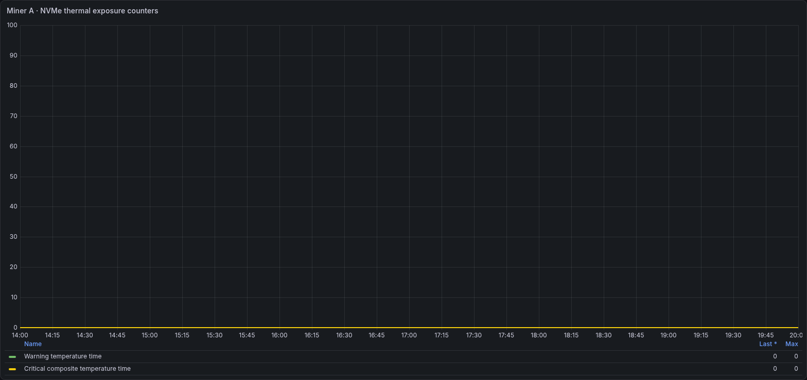
These raw counters record drive-reported thermal exposure. The gallery leaves them in exporter units rather than assuming a time conversion from their names.

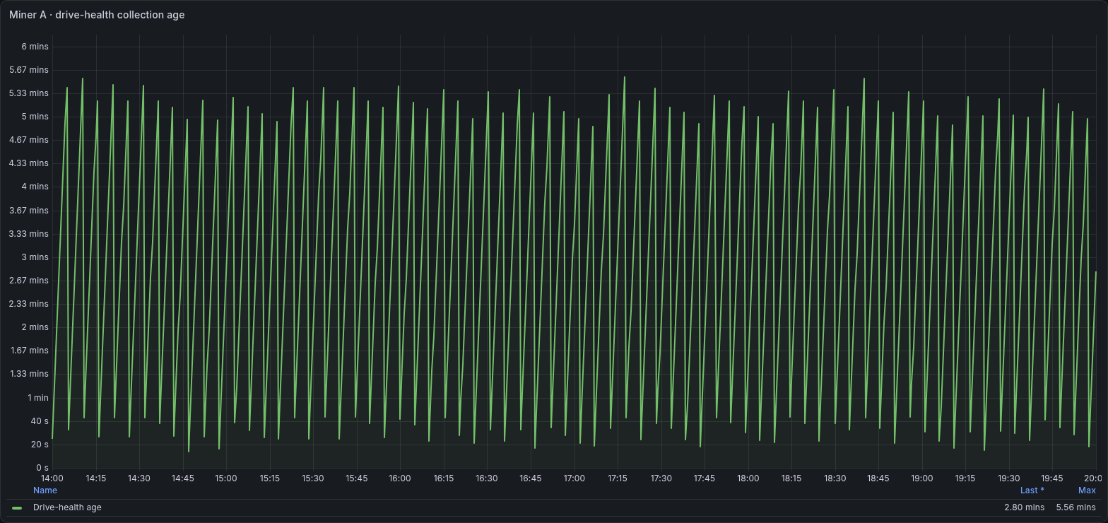
Drive health has its own collection timestamp. Check this age before treating an unchanged SMART value as a recent observation.

Next: Part 3, logs, alerts and troubleshooting

A graph can identify when a measurement changed without explaining why. Part 3 adds the journal entries and alert conditions needed to investigate that interval, then tests the path from a failed collection to a delivered notification.

Previous: Part 1, collect and store metrics.